8 Appendix
8.1 Geomorphology
8.1.1 Torrential headwater catchment
In Alpine regions, torrential processes like floods (often with high sediment transport rates) and mass movements like debris floods or debris flows are generally related to occur in small catchments with steep stream channels (torrents) prone to gravitational attraction. Thus, a mountain torrent 2 is typically associated to small headwater catchments with a steep average gradient, but the longitudinal profile consists of sections of different degrees of bed inclination.
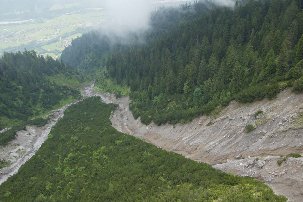
As described by K.-H. Schmidt and Ergenzinger (1994), mountain torrents might also be characterized by highly variable discharges and sediment transport volumes with bedload constituting a substantial part of the total load. Solid load transport is primarily controlled by the availability of material and the unsteady activity of sediment sources. The material supplied to sediment transport is highly irregular in grain size and angularity. Mao et al. (2009) describes a torrent as a small stream, draining steep and small (\(\leq 10 km^2\)) mountain catchments. They further highlight the presence of non-Newtonian (debris and mud) flows with an intermediate hyperconcentrated flow phase. Similar, Rickenmann (2016) characterises torrents showing channels steep enough that debris flows can occur apart from fluvial sediment transport.
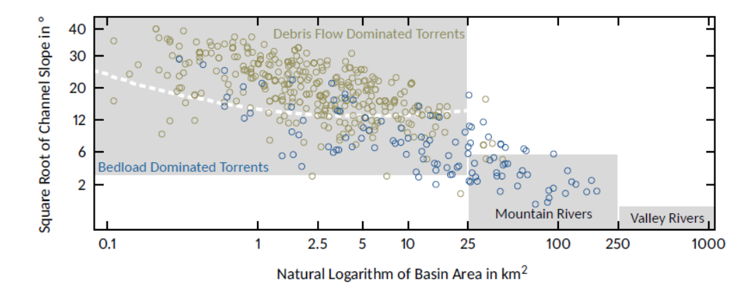
Figure 8.1: River classification, shown as grey regions according to Rickenmann, Hunzinger, and Koschni (2008). Catchments with a channel slope of at least \(3°\) and an area below \(25 km^2\) are classified as torrents. With increasing catchment area and accordingly decreasing channel slope, torrents become mountain rivers with a maximal channel slope of \(6°\) and catchment areas ranging from \(25 km^2\) to \(250 km^2\). Finally, valley rivers can be classified with catchment areas \(>250 km^2\) and channel slopes \(< 1°\). Fluvial bedload transport is beside in torrents also frequently observed in mountain rivers but not in valley rivers. Torrents can be divided in debris flow and bedload dominated catchments, which is indicated by the dashed white line. Reading example: A catchment with an area of \(25 km^2\) and a channel slope of \(6°\) is a bedload dominated torrent.
From a legislative perspective, the Austrian Forest Act (1975) defines a torrent as a natural, permanently or temporarily flowing body of water and sediment – typically situated in small, steep Alpine headwater catchments.
8.1.2 Sediment disposability
The presence of mobilised sediments of different grain sizes and quantities is a typical feature of torrential catchments and has a decisive influence on the type and formation of torrential processes as well as on its magnitude and frequency. Basically, a torrent can transport sediment either as i) dissolved load, ii) as floating or suspended material or more important iii) as bedload. The term bedload describes all sizes of material found in appreciable quantities in the channel bed. Particles move by rolling, sliding or saltation at velocities less than those of the surrounding flow (Knighton 1998). For sediment transport processes, bedload transport is a function of runoff hydraulics and channel parameters. Here, fluid and drag forces entrain particles into the flow. The main difference to debris flows and debris floods is the travel speed between the water and sediment. In sediment transport processes, coarse bedload particles move much slower than the water and are not in suspension. For debris floods or debris flows, fluid and all size of particles may travel at the same velocity, where all transported material is generally in suspension. Hungr, Leroueil, and Picarelli (2014), define debris flow as a very rapid to extremely rapid surging flow of saturated debris in a steep channel with strong entrainment of material and water from the flow path. Debris floods are typically involving more water than sediment (by volume) in the flow - compared to debris flows. Debris floods are further characterised by substantial transport of coarse sediments in contrary to hyper-concentrated flows, which are usually associated with a substantial transport of fine sediments in suspension (Scheidl and Rickenmann 2010). Observations of debris flow deposits indicate an abundant amount of unconsolidated fine to grained rock, the relocation of soil organic matter and sometimes woody debris. These observations give reason to suppose that erosion from hillslope-channel processes play an important role for the incidence and occurrence of debris flow events because they deliver sediment and organic material periodically to the main channel.
8.1.3 Hillslope-channel processes
Hillslope - channel processes refer to those processes that involve a transfer of slope-forming materials from higher to lower ground, under the influence of gravity, without the primary assistance of a fluid transporting agent. Such hillslope - channel processes can be slow or rapid, shallow or deep and include one or more of the mechanisms of creep, flow, slide or fall (Brunsden 1979). Figure 8.2 shows schematic types of hillslope failures. It is important to note that different hillslope channel failure types initiate different intensity of sediment mobilisation. For example, circular failure forms (e.g. deep seated rotational slides) or dam brake failures are characterised by mobilising a high volume of sediment in a very short time, whereas low intensities of sediment mobilisation are associated with wedge or plane failure types.
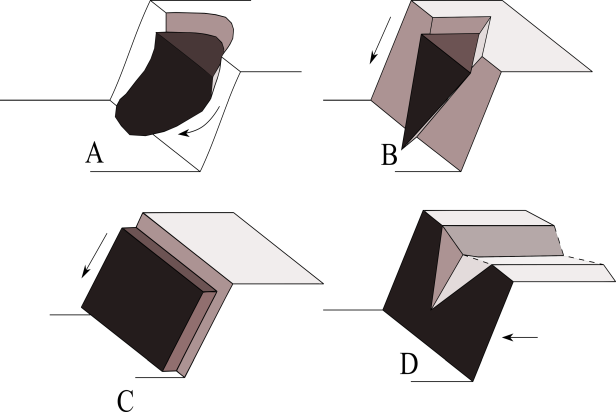
Figure 8.2: Schematic types of hillslope channel fractures. A) circular failure; B) wedge failure; C) plane failure and D) dam break failure
8.1.3.1 Infinite slope stability model
The stability of a slope is usually expressed by the factor of safety (\(FS\)), which can be calculated as the quotient of the mobilised shear strength (\(\tau_{res}\)) and the shear stress (\(\tau\)) that occurs on the sliding plane of a soil column (Fig.:8.3).
\[\begin{equation} FS=\frac{\tau_{res}}{\tau} \tag{8.1} \end{equation}\]
The shear stress (\(\tau\)) in equation (8.1) is calculated from the so-called “driving” forces per unit area which, supposing an infinitely long slope, is assumed to be \(1m^2\). The driving force is the total weight (\(G\)) acting on the sliding plane and the acting shear stress can then be expressed by the height (\(h\)) and specific density (\(\gamma\)) of the soil column, as well as by the slope angle (\(\beta\)):
\[\begin{equation} \begin{split} \tau &=G\sin\beta\\ &=h\gamma\cos\beta\sin\beta \end{split} \tag{8.2} \end{equation}\]
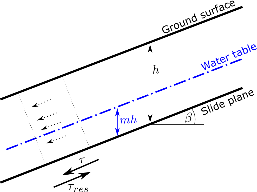
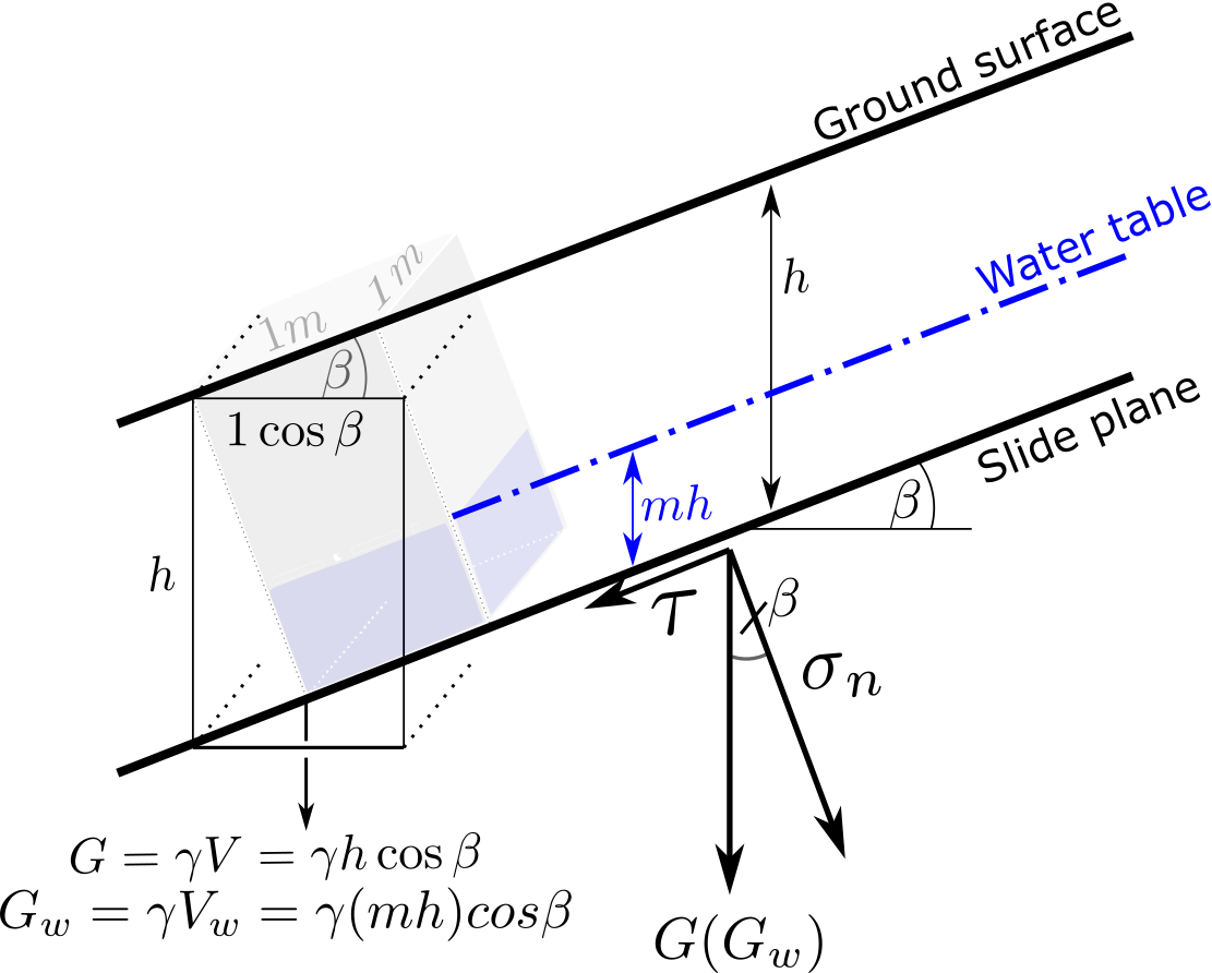
Figure 8.3: Concept of the infinite slope stability model
The shear strength (\(\tau_{res}\)) is calculated from the resistance forces per unit area and can be calculated using the concept of Coulomb:
\[\begin{equation} \tau_{res}=c'+\sigma_{eff}\tan\phi \tag{8.3} \end{equation}\]
Thus, the shear strength, acting at the sliding plane, is a function of the cohesion (\(c'\)), the effective normal stress (\(\sigma_{eff}\)) and the internal friction angle (\(\phi\)).
Here, cohesion (\(c'\)) is caused by chemical, physical and electrostatic bonding (not by compressive forces holding particles together) Apparent cohesion can either be produced by capillary stresses, occurring as surface tension in water films between particles, or by interlocking of particles at a microscopic level as a result of surface roughness or by the bonding strength of roots ([root cohesion][The role of forest on erosion control]).
Loose packing, large grain-size, high moisture contents and low wettability of particles all contribute to low cohesion.
The internal friction angle depends on the surface roughness and is the maximum angle of the resulting resistance force that must be overcome to cause sliding (Fig. 8.4).
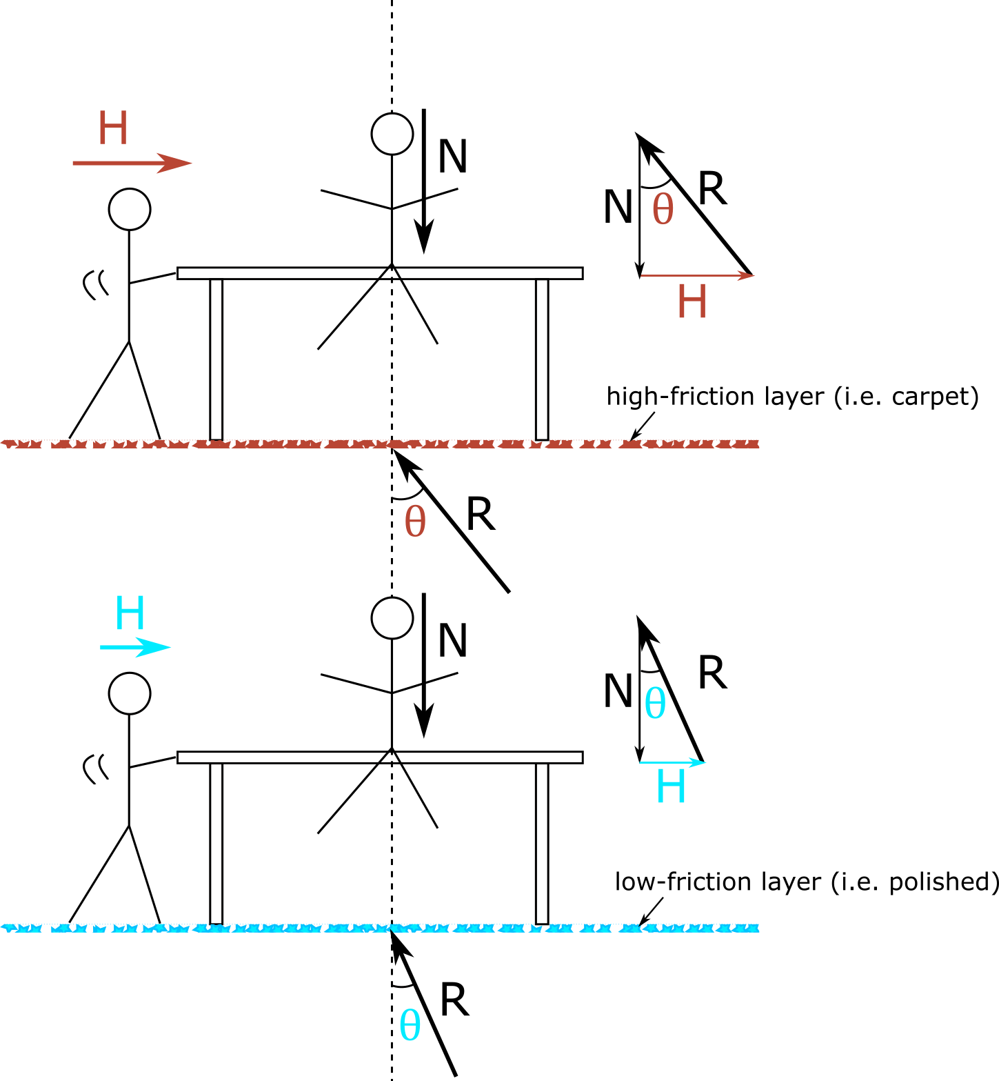
Figure 8.4: Schematic representation of the derivation of the internal friction angle
Consider a table on which a person exerts a normal force \(N\) on the floor (= sliding surface). The magnitude of the horizontal force \(H\) that must be exerted by another person to push the table away depends on the nature of the floor. The more “slippery” the floor, the lower the internal friction angle (\(\theta max = \phi\)).
\(\tan\phi\) is thus given with:
\[\begin{equation} \tan\phi=\frac{H}{N} \tag{8.4} \end{equation}\]
or substituting by shear stress (\(\tau\)) and normal stress (\(\sigma\)):
\[\begin{equation} \tan\phi=\frac{\tau}{\sigma} \tag{8.5} \end{equation}\]
The effective normal stress (\(\sigma_{eff}\)) represents the stress transmitted only through the soil skeleton. It is defined by the total force per unit area transmitted in the normal direction, respectively the total normal stress (\(\sigma_n\)), reduced by the pore pressure of the water (\(u\)) filling the cavity between the solid particles.
\[\begin{equation} \sigma_{eff}=\sigma_{n}-u \tag{8.6} \end{equation}\]
Following the annotation in Figure (8.3), the total normal stress (\(\sigma_n\)) of the soil column above the sliding plane can be defined with:
\[\begin{equation} \begin{split} \sigma_{n} &=G\cos\beta\\ &=h\gamma\cos^2\beta \end{split} \tag{8.7} \end{equation}\]
The same derivation also applies to the pore water pressure (\(u\)):
\[\begin{equation} \begin{split} u &=G_w\cos\beta\\ &=mh\gamma_w\cos^2\beta \end{split} \tag{8.8} \end{equation}\]
with (\(G_w\)) the weight and (\(\gamma_w\)) the specific weight of the pore water, and (\(m\)) the height of the water table above the sliding plane within the considered soil column (cf. Fig.:8.3).
Integrating equations (8.6) to (8.8) into (8.3) leads to:
\[\begin{equation} \tau_{res}=c'+(\gamma-m\gamma_w)h\cos^2\beta\tan\phi \tag{8.9} \end{equation}\]
Based on equations (8.2) and (8.9), the factor of safety (\(FS\)) can finally be defined by:
\[\begin{equation} FS=\frac{c'+(\gamma-m\gamma_w)h\cos^2\beta\tan\phi}{h\gamma\cos\beta\sin\beta} \tag{8.10} \end{equation}\]
For FS<1 the slope is in condition of failure. However, most natural hillslopes upon which landsliding can occur have FS values between about 1 and 1.3, but such estimates depend upon an accurate knowledge of all the forces involved. The greatest uncertainties are are usually associated with soil water (porewater pressure) (Selby 1982).
8.2 Hydrology
8.2.1 Rain and Snow
Rain and snow basically form in atmospheric clouds. Clouds consist of water droplets that condense on very small nuclei (aerosols) when the air is supersaturated with water vapor (Fig. 8.5). During this energy transformation or phase change (condensation)from vapor to water, approximately 2,500 kJ/kg of energy is released. When the raindrops reach a critical size, they fall to earth as rain.
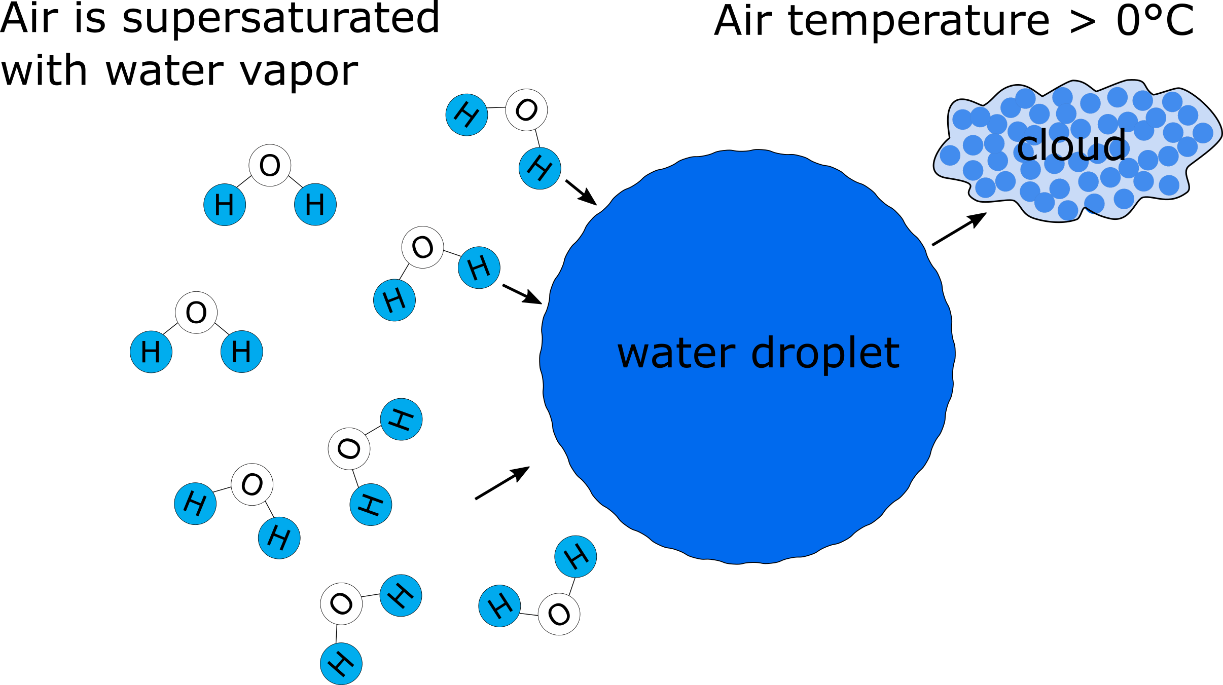
Figure 8.5: Formation of a water droplet as a component of clouds when the air is supersaturated and the air temperature is above \(0°C\)
When the air temperature at which the cloud becomes saturated is below \(0°C\), the existing water droplets become supercooled water droplets. Snow crystals can be then formed due to sublimation of water vapor from those supercooled water droplets on freezing nuclei (small ice particle, bacteria, etc). The reason why water vapour can attach to ice crystals in a saturated state has to do with the fact that the molecular bonds are weaker on a curved surface, such as a droplet, than on a flat surface. Molecules can therefore evaporate more easily from a droplet. The saturation vapor pressure is thus higher over a water droplet as compared to an ice crystal (at a given temperature)(Fig. 8.6).
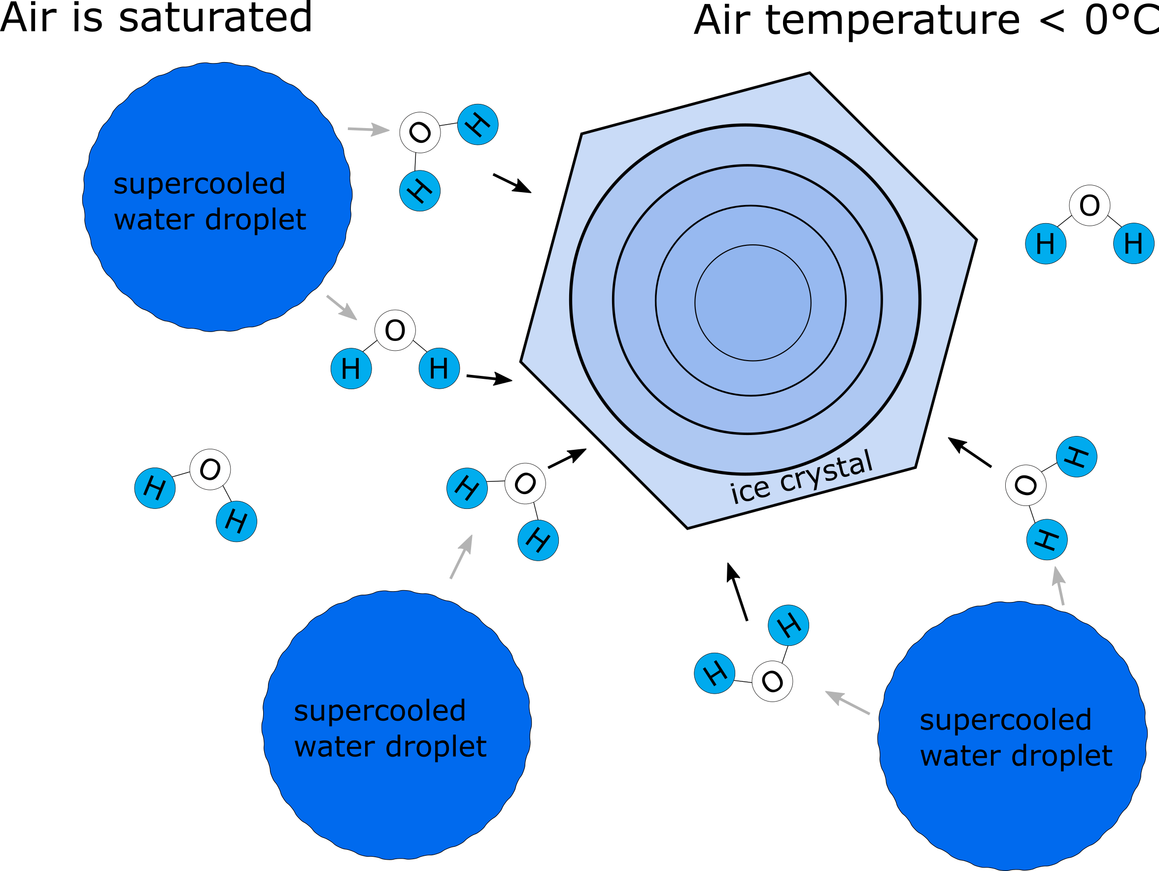
Figure 8.6: Formation of an ice crystal at saturated conditions and air temperature below \(0°C\) due to deposition of water vapor onto the ice crystal.
8.2.2 Runoff in torrents
The natural perimeter of what characterises a torrential system is typically given by its hydrological catchment 3. Generally, defined as the catchment area of precipitation or drainage basin – which drains off into a common outlet – hydrological catchments transform precipitation into outflow hydrographs, via their constituent hillslopes and channel networks (Knighton 1998). Treating a torrential system in a hydrological framework is the purpose of the research discipline Hydrology. Owing to the spatial and temporal variability of rainfall-runoff processes, a set of different hydrological transfer concepts have been established. For torrential hazard and mitigation management concepts, back-calculation or estimation of an event outflow hydrograph (Fig.:8.7) from a rainfall-runoff event is essential. The outflow hydrograph, i.e. the development of the outflow over time \(\mathit{Q(t)}\), is generally defined by two parameters: i) lag time and ii) peak flow rate or peak discharge. The later, either declared at its maximum (\(\mathit{HHQ}\)), for a distinct peak value (\(\mathit{HQ}\)), or for a certain return period (\(\mathit{HQ_T}\)).
![Schematic flood hydrograph [after @Knighton1998]](figures/hydrograph.png)
Figure 8.7: Schematic flood hydrograph (after Knighton 1998)
In many torrential catchments, however, no information about past rainfall-runoff events exists – mainly because of the lack of continuous discharge measurements devices (water gauges). In Austria, nearly 96 \(\%\) of all torrential catchments are unobserved. First attempts to estimate peak flood discharges (\(\mathit{HHQ}\), \(\mathit{HQ}\) or \(\mathit{HQ_T}\)) in torrential systems were therefore based on observed precipitation events, topographical, vegetation, soil and sometimes geomorphological parameters (Hofbauer 1916; Wundt 1953; Klement and Wunderlich 1964; Länger 1981; Bergthaler 1984). Many of those simple and empirical based approaches are still in use to check plausibility.
A common approach to estimate peak discharge without knowing the corresponding runoff is based on the rational method (Kuichling 1889). Estimation of a maximum discharge \(\mathit{HQ_T}\) is based on the following equation, \[\begin{equation} HQ_T=0.278A_{c} C_r i_T \tag{8.11} \end{equation}\] with the drainage area \(A_{c}\), a rational runoff coefficient \(C_r\) and \(i_T\) the rainfall intensity for a certain recurrence interval. The runoff coefficient \(C_r\) is defined as the ratio between effective precipitation (transferred to discharge) and total precipitation. Based on rainfall simulations in different torrential catchments throughout Austria with a rainfall intensity of 100mm/h, Kohl (2011) showed that in 38\(\%\) of all simulation sites half of the total precipitation is transferred to runoff (\(C_r\geq 50\%\)). He further observed Horton overland flow, which means that the rainfall has exceeded soil infiltration capacity, in 58\(\%\) of all simulation sites. Only for 19\(\%\) of all test sites, soil infiltration capacity was higher than simulated rainfall intensity. Rainfall intensity \(i_T\) is a function of rainfall duration \(D\), rainfall return interval \(T_r\) and time of concentration \(t_c\). The time of concentration is defined as the time a water particle needs (without any significant soil storage) from the outermost point of the watershed to the area outlet. In general, it can be expressed as: \[\begin{equation} t_c=a {L_{flow}}^b {n_r}^c {S}^d {i_T}^e \tag{8.12} \end{equation}\] In equation (8.12), \(L_{flow}\) denotes to the length of flow, \(S\) the slope, \(n_r\) reflects to the resistance to flow (e.g.: Kerby, Manning or Izzard roughness coefficients) and \(a\) to \(e\) are empirical parameters. The concept assumes a uniformly constant rainfall over the entire catchment area whereas maximum discharge will be reached when the duration of precipitation equals or exceeds the characteristic time of concentration. For this reason, it is predestined for small steep headwater catchments where convective (heavy) rainfall events are dominant.
A sound overview of hydrological approaches to estimate runoff formation in torrential catchments can be found in Hagen, Ganahl, and Hübl (2007) and more recently in Rimböck et al. (2013).
8.2.3 Runoff transfer concepts
Recently, hydrological models might be classified as lumped or distributed models with any specifications in between. Lumped models treating the complete basin as a homogeneous whole, whereas semi-distributed models attempt to calculate flow contributions from separate areas or sub-basins that are treated as homogeneous within themselves. Fully distributed models divide the whole basin into elementary unit areas like a grid net and flows are passed from one grid point (node) to another as water drains through the basin (Xu 2002). Like in many other scientific disciplines hydrological models can further be divided in stochastic, empirical (black-box, input-output models), conceptual (grey-box models) and theoretical (or physically-based, white box models) approaches.
A widespread method to estimate \(Q_f(t)\) is based on the instantaneous unit hydrograph theory (IUH), a transfer function based on a precipitation impulse of 1mm with a duration of \(d_\tau\). For torrential systems, \(Q_f(t)\) can be expressed by combining hillslope reponse function and a network reponse function (e.g. Knighton 1998; Gupta and Mesa 1988; Rigon et al. 2016):
\[\begin{equation}
Q_f(t)=\int_{0}^{t}q_h(t-\tau)q_n(\tau)d_\tau
\tag{8.13}
\end{equation}\]
The determination of a unit hydrograph for a certain torrential catchment depends, however, on information about observed rainfall-runoff events.\
Conceptual models use a water balance approach considering transfer of rainfall into direct runoff “conceptually” as equivalent to transferral through a series of reservoirs linked by channels. Conservation of mass for the entire catchment is then given by the catchment water balance,
\[\begin{equation}
Q_f(t)=P(t)-E(t)-T(t)-\frac{dS}{dt}
\tag{8.14}
\end{equation}\]
with \(P\) precipitation, \(E\) evaporation, \(T\) transpiration and \(S\) water storage.
8.3 Avalanches
8.3.1 Classification according to starting area
Avalanches can be divided into either loose snow avalanches or snow slab avalanches according to the shape of the starting area. The characteristic of a loose snow avalanche results from the fact that it starts at a single starting point and spreads downwards (Fig.:8.8).
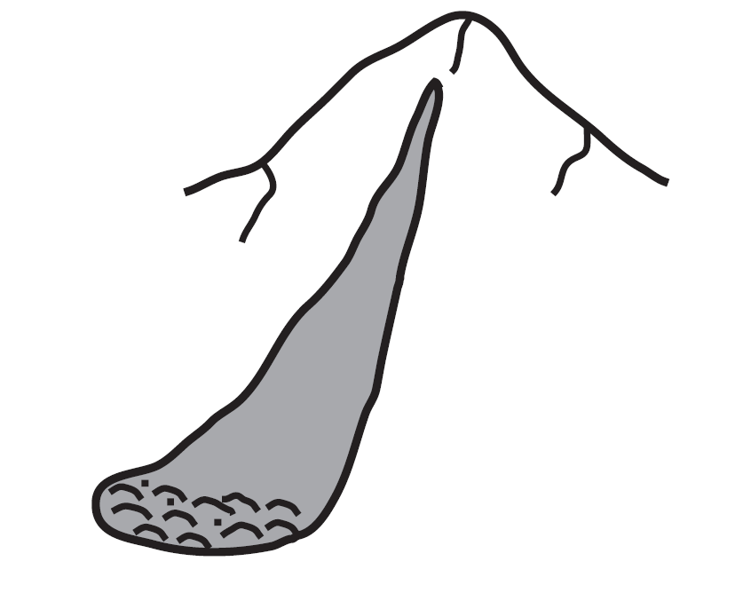
Figure 8.8: Shape of a loose snow avalanche
A snow slab avalanche, on the other hand, begins with a fracture in the depth of the snowpack, which usually has a rectangular shape (Fig.:8.9).
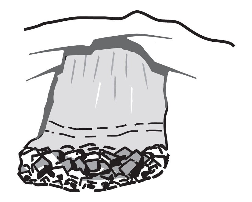
Figure 8.9: Shape of a slab avalanche
8.3.2 Classification according to the way of motion
Here one differentiates between airborn powder snow avalanches and dense (flowing) avalanches. Airborn powder snow avalanches are characteristed if a powder cloud forms in the presence of a large altitude difference when a sufficient quantity of snow becomes suspended in the air (Fig.:8.10). In this case, the powder avalanche may completely lose contact with the ground surface, rendering the topography or structural protective measures in the transit route (deflection dams, brake barriers, etc.) ineffective.
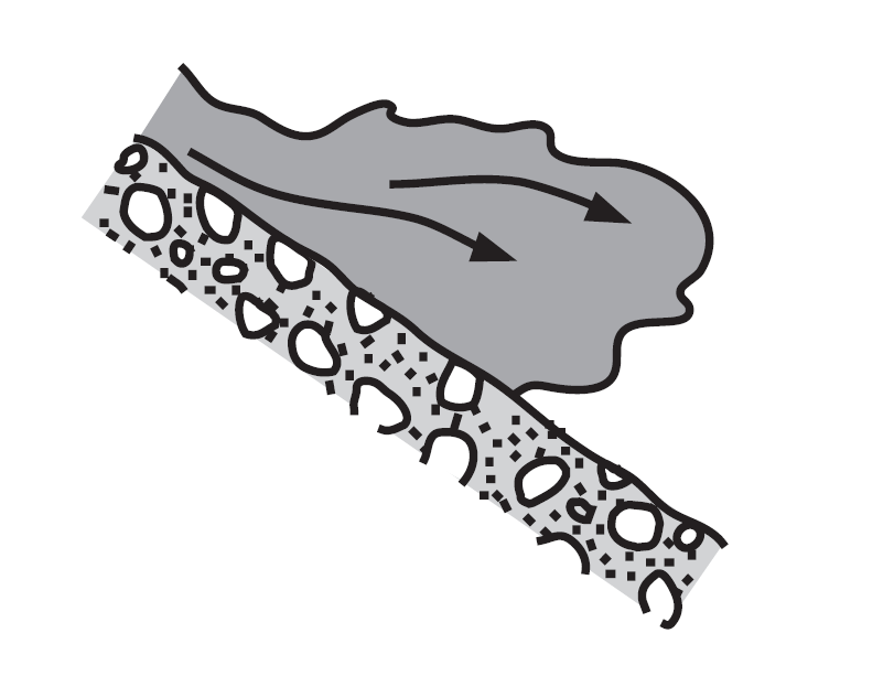
Figure 8.10: Shape of a slab avalanche
In contrast, the (denser) mass of a dense flowing avalanche always moves close to the ground and follows the local topography.
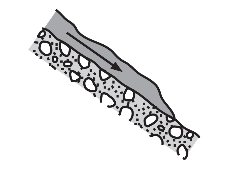
Figure 8.11: Shape of a slab avalanche
8.3.3 Classification according to the location of the sliding surface
If the rapture zone lies within the snow cover, it is called a surface layer avalanche (Fig.:8.12).
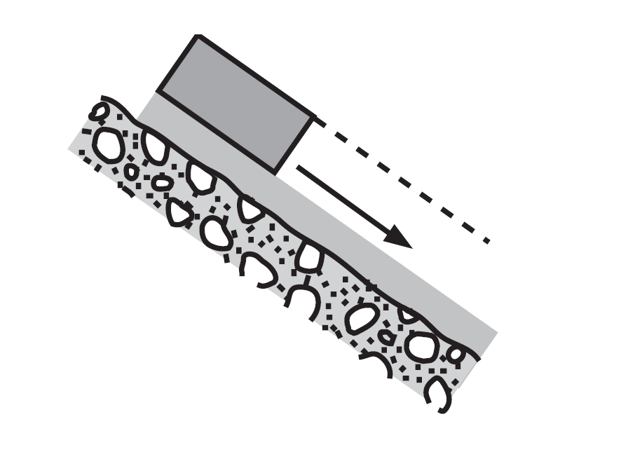
Figure 8.12: Shape of a slab avalanche
If the sliding surface is on the ground, it is called a full layer or ground avalanche (Fig.:8.13).
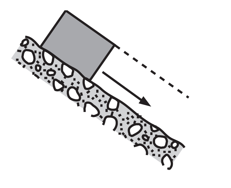
Figure 8.13: Shape of a slab avalanche
8.4 Math
8.4.1 Probability
The probability is generally defined as the quotient of the number of cases in which a specific event occurs and the number of possible cases. It varies between \(0\) (occurrence impossible) and \(1\) ( occurrence).
Example 8.1 \iffalse (Bernoulli experiment) A random experiment is a process in which exactly two outcomes are possible and in which the result can not foresee before the end of the process. One of the test outputs is designated with success (\(1\)) and the complementary experiment defined with failure (\(0\)). The associated probability of success is called probability of success \(p\) and \(q = 1-p\) the probability of failure.
Question: What is the likelihood of an event?
Example: What is the probability that a snow depth is greater than a certain 3-day new snow sum with a return period of 50 years?
\[\begin{equation} p=\frac{1}{50}=0.02 \end{equation}\] \[\begin{equation} q=1-p=0.98 \end{equation}\]Example 8.2 \iffalse (Conditional probabilities) If events A and B are independently of one another the following applies:
\[\begin{equation} p(A \cap B)=p(AB)=p(A)p(B) \end{equation}\] \[\begin{equation} p(A \mid B)=\frac{p(A)p(B)}{p(B)}=p(A) \end{equation}\]
Question: What is the probability of a \(T\) - annual event in \(n\) consecutive years ?
Example : What is the probability that an avalanche with a return period of 50 years occurs within two consecutive years?
1. year: \(p(A)=\frac{1}{50}\)
2. year: \(p(B)=\frac{1}{50}\)
\[\begin{equation} p(AB)=p(A)p(B) \implies p(A)=p(B)=\frac{1}{50} \implies p(AB)={\left( \frac{1}{50}\right) }^2=0.0004 \end{equation}\]8.4.2 Return period
With the return period (frequency, recurrence interval), the recurrence probability of natural events is described. It is defined as the average time, of he occurrence of an event, required (\(T\)) for which the intensity (\(Q\)) reaches or exceeds a threshold value (\(QT\)) (reciprocal of exceedance probability \(P_e\)). \[\begin{equation} P_e=P(Q \geq Q_T)=\frac{1}{T} \text{ respectively } \frac{100}{T} [\%] \end{equation}\] \[\begin{equation} \text{ with } T=\frac{1}{P_{ne}} \end{equation}\]
Theorem 8.1 An event with 100 – year return period is statistically reached or exceeded once in 100 years, so it might statistically occur 10 times in 1000 years. Thus, this event has an average return period of 100 years (\(T\) = 100 a), an exceedance probability \(P_u\) of 0.01, or 1 \(\%\), and a non-exceedance probability \(P_{ne}\) of 0.99 or 99 \(\%\), so it does not occur, on average, in 99 out of 100 years.
8.5 Forest parameters
8.5.1 Leaf Area Index (LAI)
Leaf Area Index (LAI) was defined by Watson (1947) as the total one‐sided area of leaf tissue per unit ground surface area. According to this definition, LAI is a dimensionless quantity characterizing the canopy of an ecosystem. Leaf area index drives both the within‐ and the below‐canopy microclimate, determines and controls canopy water interception, radiation extinction, water and carbon gas exchange and is, therefore, a key component of biogeochemical cycles in ecosystems. Any change in canopy leaf area index (by frost, storm, defoliation, drought, management practice) is accompanied by modifications in stand productivity. Process‐based ecosystem simulations are then often required to produce quantitative analyses of productivity and LAI is a key input parameter to such models (Bréda 2003)